A Practical Guide to Neural Network Quantization

Modern artificial intelligence, particularly Deep Neural Networks (DNNs), has achieved remarkable feats across various domains, from image recognition to natural language processing. However, this power comes at a significant cost of immense computational and energy requirements. This challenge is especially pronounced with the growing demand to deploy AI directly on edge devices - compact, resource-constrained hardware like smartphones, smartwatches, and automotive systems. To bridge this gap, techniques that enhance model efficiency are crucial. Among these, Neural Network Quantization stands out as a powerful and practical solution.

This post delves into the intricacies of neural network quantization, explaining its fundamental principles, diverse methodologies, and profound benefits for enabling efficient AI at the edge.

The Energy Hunger of Deep Neural Networks

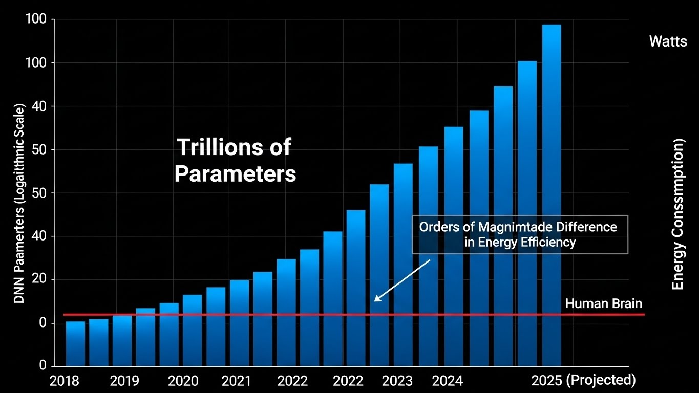
Deep Neural Networks are rapidly increasing in complexity and scale. In 2021, some DNNs reached 1.6 trillion parameters, with projections indicating a staggering 100 trillion parameters by 2025. This exponential growth translates directly into colossal energy consumption. Compared to the human brain, which operates with remarkable efficiency, DNNs are estimated to be about 100,000 times less energy-efficient. This disparity highlights a critical barrier to sustainable and widespread AI deployment.

The Shift to Edge AI and its Constraints

The ability to process AI workloads directly on edge devices is transforming industries by enabling real-time insights, enhanced privacy, and operation without constant cloud connectivity. However, these devices operate under severe constraints:

• Limited Compute Resources: CPUs and GPUs on edge devices are far less powerful than their data center counterparts.
• Complex Concurrency: Managing multiple tasks simultaneously efficiently is challenging.
• Real-time Processing: Many applications (e.g., autonomous driving) demand instantaneous responses.
• "Always-on" Requirements: Devices like smart assistants need to be constantly ready, requiring extremely low power states.
• Strict Thermal and Power Budgets: Heat dissipation and battery life are major design considerations.

A significant power bottleneck in neural network execution on these devices is the data transfer between memory and compute units. Moving data around consumes substantially more energy than performing arithmetic operations.

Neural Network Quantization: The Core Solution

To address the efficiency challenges of DNNs on edge devices, AI research focuses on several key techniques, including compression, quantization, and compilation. Among these, quantization stands out as a particularly effective method for reducing power consumption and improving performance.

What is Neural Network Quantization?

At its core, neural network quantization is a technique that reduces the precision of the numerical representations used for storing model weights and performing computations. Instead of using high-precision data types, such as FP32 (32-bit floating-point numbers), quantization employs lower bit-width integers, commonly INT8 (8-bit integers).

Think of it like reducing the number of colors in an image. An image stored with 24 bits per pixel can display millions of colors (high precision). Reducing it to 8 bits per pixel significantly reduces file size and processing load while still maintaining acceptable visual quality for most purposes. Similarly, quantization approximates the detailed floating-point values of a neural network with a fixed number of integer levels.

Significant Benefits of Quantization

The adoption of lower bit-widths through quantization yields substantial advantages for edge deployment:

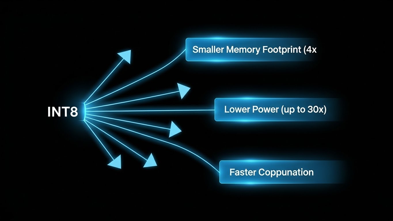
• Memory Usage: Storing weights and activations in 8-bit integers requires 4 times less memory compared to 32-bit floating-point numbers. This reduces model footprint and eases memory bandwidth constraints.
• Power Consumption: Lower bit-width computations are significantly more energy-efficient. For instance, an 8-bit integer addition can be 30 times more energy-efficient than a 32-bit floating-point addition, and an 8-bit integer multiplication 18.5 times more efficient. Memory access power consumption can also be reduced by up to 4 times.
• Latency: Fewer memory accesses and simpler fixed-point arithmetic operations lead to faster inference times, crucial for real-time applications.
• Silicon Area: Integer arithmetic units require less dedicated silicon area on integrated circuits. For example, 8-bit integer adders can be 116 times smaller than FP32 adders, and multipliers 27 times smaller. This translates to more compact and cost-effective hardware designs.

Understanding Quantization: How It Works

The fundamental idea behind quantization is to approximate a high-precision floating-point tensor, let's call it X, using a lower-precision integer tensor, X_int. This approximation is achieved through a simple linear mapping:

X = s_X * X_int

Here, s_X is a scale factor, a floating-point number that maps the integer range to the desired floating-point range. X_int represents the quantized integer values.

The core operation in most neural networks is matrix multiplication (e.g., WX + b, where W are weights, X are inputs, and b is bias). Modern hardware accelerators for AI often utilize MAC (Multiply-Accumulate) arrays to perform these operations efficiently in parallel.

During quantized inference:

1. Weights (W) and inputs (X) are converted from their original floating-point representation to low-precision integers, typically UINT8 (unsigned 8-bit integer, values 0-255) or INT8 (signed 8-bit integer, values -128 to 127).
2. The MAC arrays then perform integer multiplications and additions.
3. To prevent overflow during the accumulation of intermediate sums, the accumulators (the registers that hold these sums) often use a higher bit-width, commonly INT32 (32-bit integer). This ensures that the sum of many small 8-bit products does not exceed the maximum representable value before the final de-quantization step.

graph TD
A[FP32 Tensor W] --> B[Quantize W INT8]
C[FP32 Tensor X] --> D[Quantize X INT8]
B -- Multiply --> E[MAC Array]
D -- Accumulate --> E
E -- Result (INT32 Accumulator) --> F[Dequantize Result FP32]
F --> G[Next Layer / Output]

The Trade-off: Lost Precision (Quantization Noise)

While quantization offers significant advantages, it is not without a cost. The process of mapping continuous floating-point values to discrete integer levels inherently introduces an approximation error, often referred to as "quantization noise." This error (epsilon = W - s_W _ W_int) can degrade the accuracy of the neural network.

The field of quantization research is heavily focused on two primary goals:

1. Minimizing this quantization noise.

2. Developing neural networks that are more robust and resilient to this introduced error, thereby maintaining high accuracy even at very low bit-widths.

Types of Quantization: Grids and Granularity

Quantization methods are broadly categorized based on how the fixed-point grid is defined and how widely it is applied across the network.

Fixed-Point Grids

A fixed-point grid is characterized by a scale factor (s) and a zero-point (z). These parameters define how floating-point numbers are mapped to their integer representations.

• Scale Factor (s): Determines the spacing between adjacent quantization levels. A smaller s means finer granularity within the same integer range.
• Zero-Point (z): An integer value that maps the floating-point zero to a specific integer value.

The choice of s and z significantly impacts the quantization error.

Symmetric Quantization (z = 0)

In symmetric quantization, the floating-point zero is directly mapped to the integer zero. This simplifies calculations as the zero-point term effectively vanishes.

• Symmetric Signed (INT8): Uses a range like -128 to 127. This is ideal for distributions of values (like model weights) that are often centered around zero and exhibit a relatively symmetric distribution.
• Symmetric Unsigned (UINT8): Uses a range like 0 to 255. This is well-suited for activations after a ReLU (Rectified Linear Unit) function, which clips negative values to zero, resulting in a skewed distribution that is predominantly positive.

Asymmetric Quantization (z != 0)

Asymmetric quantization is more flexible, allowing the floating-point zero to map to any integer zero-point without error. This can offer a better distribution of quantization error for certain activation patterns by aligning the quantization range more precisely with the data's dynamic range.

The trade-off is increased computational overhead during inference, as the non-zero z introduces additional terms in the calculations. These terms either need to be precomputed (e.g., folded into the bias) or incur data-dependent overhead.

Choosing the Right Quantization Type

• Symmetric quantization is generally simpler to implement in hardware due to fewer terms in the underlying mathematical operations.
• Asymmetric quantization, while more flexible, introduces additional computational complexity.

Quantization Granularity

Beyond the type of grid, how consistently the (s, z) parameters are applied across a tensor (a multi-dimensional array of numbers used to represent data in a neural network) is another crucial aspect.

• Per-tensor Quantization: A single (s, z) pair is applied to the entire tensor.
  • Pros: Simplest to implement, widely supported by fixed-point hardware accelerators.
  • Cons: May not optimally utilize the quantization range if the tensor has a wide dynamic range or highly varied distributions within different parts (e.g., different channels of a convolutional layer).
• Per-channel Quantization: A unique (s, z) pair is determined for each channel within a tensor. For example, in a convolutional layer with 64 output channels, there would be 64 distinct (s, z) pairs for its weights.
  • Pros: Better utilizes the available quantization grid by adapting to the specific dynamic range of each channel, potentially reducing quantization noise and improving accuracy. This is particularly effective for addressing the "imbalanced weights" problem, where some channels have significantly larger dynamic ranges than others.
  • Cons: Requires specific hardware support for efficient implementation, as processing multiple (s, z) pairs simultaneously adds complexity. Increasingly popular for weights.

Feature	Per-tensor Quantization	Per-channel Quantization
(s, z) Application	One pair for the entire tensor	One unique pair for each channel
Complexity	Low (simple hardware implementation)	Moderate (requires specific hardware support)
Accuracy Potential	Good, but can be limited	Generally higher (better range utilization)
Use Case	Common for activations, weights (simpler hardware)	Increasingly common for weights (imbalanced distributions)
Hardware Support	Widely supported	Growing, but not universal

Simulating Quantization

Testing quantized models directly on edge hardware can be a time-consuming and expensive process. To accelerate development and experimentation, quantization simulation is a vital step.

Why Simulate?

Simulation allows developers to:

• Rapidly experiment with different quantization options (e.g., bit-widths, types of quantization).
• Estimate the accuracy impact of quantization without needing to deploy to physical hardware.
• Debug quantization-related issues in a controlled environment.

How it Works

Quantization simulation is performed on general-purpose floating-point hardware (like a CPU or GPU) by inserting explicit "quantizer" operations into the neural network's compute graph. These quantizer operations mimic the behavior of fixed-point arithmetic.

A typical quantizer operation involves two steps:

1. Quantization: X_int = clip(round(X/s) + z, min=0, max=2^b-1)
   • The floating-point value X is scaled by 1/s, shifted by z, and then rounded to the nearest integer.
   • clip ensures the value stays within the target bit-width b's integer range (e.g., 0 to 255 for UINT8).
2. De-quantization: X_hat = s * (X_int - z)
   • The integer X_int is converted back to an approximate floating-point value X_hat using the same scale factor and zero-point. This X_hat is then used for subsequent floating-point computations in the simulated environment.

Sources of Error

Simulation also highlights the two primary sources of error introduced by quantization:

• Rounding Error: Occurs because floating-point values are rounded to the nearest integer within the defined grid.
• Clipping Error: Occurs when floating-point values fall outside the chosen quantization range, and are therefore "clipped" to the minimum or maximum representable integer value.

There is often a trade-off between these two errors: extending the range to reduce clipping might increase rounding error for values closer to the center, and vice versa.

graph LR
A[FP32 Input Tensor] --> B[Quantize Operation]
B --> C[Integer Tensor Simulated]
C --> D[Dequantize Operation]
D --> E[FP32 Approximate Tensor]
E --> F[Standard FP32 Operations]
B -- Error Introduced --> G[Rounding Error]
B -- Error Introduced --> H[Clipping Error]

Choosing Quantization Parameters (Calibration)

A critical step in quantization is determining the optimal (s, z) parameters, which define the mapping from floating-point to integer values. This process is called calibration.

• Min-max Range: The simplest approach, where q_min and q_max are simply the minimum and maximum observed floating-point values in a representative dataset. This method is straightforward but can be sensitive to outliers.
• Optimization-Based Methods: More advanced techniques treat the choice of q_min and q_max as an optimization problem. They aim to argmin(L(X, X_hat(q_min, q_max))), minimizing a loss function (e.g., Mean Squared Error (MSE) or Cross-entropy loss) between the original and quantized tensor. These generally yield better accuracy for activations.
• Batch-Norm Based Methods: For certain network architectures, especially those using Batch Normalization (BN) layers, it's possible to infer quantization ranges in a data-free manner. This method leverages the statistical parameters of the batch normalization layer and makes assumptions about the Gaussian distribution of pre-activation values.

Quantization Algorithms: PTQ vs. QAT

The two main categories of quantization algorithms are Post-Training Quantization (PTQ) and Quantization-Aware Training (QAT). They differ significantly in their approach, data requirements, and achievable accuracy.

Post-Training Quantization (PTQ)

PTQ converts a pre-trained, full-precision (FP32) neural network into a fixed-point network after training is complete, without further retraining.

• Process:
  1. Train the neural network in full precision.
  2. Use a small, unlabeled dataset (calibration set) or no data at all to determine the quantization parameters (s, z) for weights and activations.
  3. Convert the model to its quantized (e.g., INT8) equivalent.
• Data Requirements: Can be entirely data-free for weights, or require only a small, unlabeled calibration set for activations.
• Ease of Use: Typically involves a single API call in quantization frameworks.
• Challenge: Can sometimes lead to a noticeable drop in accuracy, especially at very low bit-widths (e.g., 4-bit weights), as the network was not originally trained to be robust to quantization noise.

Key PTQ Techniques:

• Cross-Layer Equalization (CLE): Addresses issues arising from "imbalanced dynamic ranges" between adjacent layers. CLE scales the weights of neighboring layers to harmonize their dynamic ranges, improving overall quantization quality without affecting the model's FP32 behavior. This is crucial when some channels have much larger value ranges than others.
• Bias Correction: Compensates for systematic "bias" or error introduced by the quantization process, particularly for weights. This can often be done in a data-free manner by analyzing the distribution of quantization errors.
• AdaRound (Adaptive Rounding): A data-driven method that learns optimal rounding decisions for each weight. Instead of simply rounding to the nearest integer, AdaRound adjusts rounding (up or down) to minimize a local L2 loss. This significantly boosts accuracy, especially at challenging low bit-widths, by making small, data-aware adjustments to the quantized weights.

graph TD
A[Pre-trained FP32 Model] --> B{Collect Calibration Data Optional}
B --> C[Determine Quantization Parameters s, z]
C --> D[Apply Quantization to Weights/Activations]
D --> E[PTQ Quantized Model e.g., INT8]

Quantization-Aware Training (QAT)

QAT integrates the quantization process directly into the training loop. This means the model "learns" to be robust to quantization noise during training.

• Process:
  1. Initialize a pre-trained FP32 model.
  2. During training, simulate fixed-point arithmetic for both forward and backward passes.
  3. The network's weights are adjusted to compensate for the simulated quantization effects.
• Requirements: Requires access to the full training pipeline, including labeled training data.
• Training Time: Generally leads to longer training times and may require more hyperparameter tuning compared to PTQ.
• Accuracy: Achieves the highest accuracy among quantization methods, often recovering near FP32 performance, even at very low bit-widths.

Key QAT Concepts:

• Simulating Backward Pass (Straight-Through Estimator - STE): Quantization operations (rounding and clipping) are non-differentiable, meaning standard backpropagation cannot compute gradients directly. The Straight-Through Estimator (STE) approximates these gradients, allowing the network to learn effectively despite the discrete nature of quantization. It essentially treats the quantization operation as an identity function during the backward pass.
• Learnable Quantization Parameters: The scale factors (s) and zero-points (z) can also be learned during training through optimization, alongside the model weights. This further fine-tunes the quantization mapping for optimal performance.
• Batch-Norm Folding: Batch Normalization (BN) layers normalize the activations, which helps stabilize training. For faster and more efficient inference on quantized models, BN layers can be "folded" (merged) into adjacent convolutional or fully connected layers by pre-computing their effects into the weights and biases. This eliminates the need for separate BN computations during inference.
• Importance of Initialization: Proper initialization of quantization parameters (e.g., using PTQ techniques like CLE as a pre-processing step before QAT) is crucial, especially for models with complex architectures like depth-wise separable convolutions (common in MobileNetV2), to prevent accuracy collapse.

graph TD
A[FP32 Model Initialization] --> B{Insert Quantization Nodes Simulated}
B --> C[Forward Pass with Simulated Quantization]
C --> D[Calculate Loss]
D --> E[Backward Pass STE for Quantization Nodes]
E --> F[Update Weights and Quantization Parameters]
F -- Iterations --> C
F -- Training Complete --> G[QAT Quantized Model e.g., INT8]

PTQ vs. QAT Comparison

Feature	Post-Training Quantization (PTQ)	Quantization-Aware Training (QAT)
Training Requirement	None (applied after training)	Full training with quantization simulation
Data Requirement	Data-free or small calibration set	Full labeled training dataset
Ease of Use	Very easy (often single API call)	More complex (integrates into training loop)
Accuracy	Good, but potential degradation at low bit-widths	Highest (recovers near FP32 accuracy)
Training Time	Minimal (no additional training)	Longer (training with quantization simulation)
Hardware Implication	Can apply to any pre-trained model	Requires differentiable quantization (STE)
Best For	Quick deployments, scenarios without training data, initial accuracy checks	Achieving maximum accuracy on quantized models, low bit-widths

Real-World Impact and Open-Source Tools

The advancements in neural network quantization are not merely theoretical; they are driving the practical deployment of sophisticated AI on countless devices.

A notable open-source toolkit facilitating this is AIMET (AI Model Efficiency Toolkit) by Qualcomm. AIMET provides a comprehensive suite of state-of-the-art quantization and compression techniques. It is available on GitHub and supports both TensorFlow and PyTorch frameworks, designed to integrate seamlessly into a developer's workflow. Key features include quantization simulation, sophisticated range setting, data-free quantization methods, and advanced techniques like AdaRound. AIMET also offers other compression techniques, such as Spatial SVD and channel pruning.

Accompanying AIMET is the AIMET Model Zoo, which offers accurate pre-trained 8-bit quantized models for a wide range of popular architectures (e.g., ResNet-50, MobileNet, EfficientNet, SSD MobileNet-V2, RetinaNet, DeepLabV3+, DeepSpeech2) in TensorFlow and PyTorch. These models demonstrate that it's possible to achieve INT8 models with less than 1% accuracy loss compared to their FP32 baselines, validating the effectiveness of these quantization techniques.

Quantization Challenges and Solutions

Despite these advancements, optimizing multi-bit quantized networks remains complex due to the vast number of potential configurations. Thorough validation, often involving large datasets like the entire ImageNet validation set with hundreds of stochastic samples, is necessary to gauge the robustness and performance across diverse scenarios.

General best practices include designing quantization ranges that encompass zero to minimize error, especially for sparse activations or weights. Techniques like weight equalization and bias correction are highly recommended to mitigate and recover errors, particularly those that propagate through layers and affect activations. For recurrent neural networks (RNNs), quantizing all inputs, gate outputs, and hidden states is typical, with careful consideration for error propagation over time steps.

The ultimate output of such optimization tools is an optimized AI model, which includes the new, quantized weights along with their corresponding quantization encoding parameters, making them ready for efficient on-device inference.

Conclusion

Neural network quantization is an indispensable technique for the practical deployment of deep learning models on resource-constrained edge devices. By intelligently reducing numerical precision, it dramatically improves memory efficiency, power consumption, latency, and hardware footprint, all while striving to preserve the model's accuracy.

The choice between symmetric and asymmetric quantization, per-tensor or per-channel granularity, and algorithms like Post-Training Quantization (PTQ) or Quantization-Aware Training (QAT) depends on the specific application, hardware target, and desired accuracy-efficiency trade-offs. With robust open-source tools like AIMET, developers are increasingly empowered to navigate these complexities, delivering high-performing and energy-efficient AI solutions to the edge.

Further Reading

• Deep Learning Model Optimization Techniques
• Hardware Accelerators for AI
• Memory Management in Embedded Systems
• Fundamentals of Floating-Point vs. Fixed-Point Arithmetic
• Low-Power AI Design Principles